Introduction
Motivation
Uncertainty in engineering simulation
Since the advent of the computer, engineering simulation has become an invaluable tool for the design and analysis of systems. Simulation allows engineers to bridge the gap between theoretical models of systems and empirical evidence, whilst making predictions about yet to be constructed systems [130]. Some important applications of this include structural engineering [86], aeronautical structures [86], and petroleum reservoir engineering [13].
The engineer’s theoretical model of the system’s physics can be defined by a mathematical function or a more complex simulation, and this theoretical model will depend upon associated parameters which determine the specific properties of the system under consideration. The physical model to be used may be motivated by the engineer’s expert judgement, or prescribed by a relevant design standard document. Provided the model’s parameters are known, the model can be used to make predictions about the system. In some cases, e.g. well known material properties, the parameters to be used will also be prescribed by the design standard document. If this is not the case, the engineer must identify these parameters from data or expert judgement. Hence, in many realistic situations these parameters will not be known exactly, and therefore will be associated with some uncertainty. If the system is not well understood, then the theoretical model of the system’s physics may itself be uncertain. However, in many cases this situation can be dealt with by adding more uncertain parameters to the model, thereby increasing the model’s degrees of freedom. This uncertainty will be reflected in the predictions made by the model, hence the ability of the system to meet some specified objective, e.g. safe operation, now becomes uncertain. In essence, this motivates the well known structural reliability analysis problem, where we wish to calculate the probability that the system under uncertainty doesn’t meet a specified objective, which is referred to as the failure probability of the system [106].
Reliability engineering
Researchers in the discipline of reliability engineering have proposed many techniques to solve the reliability analysis problem. Most generally, Monte Carlo simulation can solve any reliability analysis problem with arbitrary accuracy, given sufficient samples of the uncertain system parameters and evaluations of the system model [106]. If the failure probability of the system is small, which is typical in most realistic engineering problems, then the number of model evaluations required increases significantly, and creates a bottleneck to the calculation. Therefore, in practice, more efficient methods are required to solve the reliability analysis problem for expensive computational models with many inputs. These include approximate methods, e.g. the First Order Reliability Method (FORM) and advanced simulation techniques, e.g. line sampling, which require fewer samples of the system model [86] [26].
Alternatively, since the cost of the analysis depends strongly upon the cost of evaluating the system model, one may attempt to replace the expensive system model with a cheaper surrogate, known as a metamodel. This metamodel is usually obtained by using machine learning technologies to learn a function which is a sufficiently accurate representation of the true model. Well known metamodels applied in reliability engineering include neural networks, response surfaces (polynomial regression), polynomial chaos, and Kriging (Gaussian process emulators) [86] [85] [132]. If the metamodel is inaccurate then this can introduce additional uncertainty into the calculation, and typically this must be traded off against time required to create the metamodel. In any case, the uncertainty in the metamodel should be quantified and its influence on the failure probability of the system stated. As such, the problem is challenging and does not yet have an entirely satisfactory solution, although significant progress has been made in recent years.
Models of uncertainty
Many techniques exist for modelling uncertainty, and therefore the chosen uncertainty model is also, to an extent, an engineering judgement. This judgement is usually based on the type of uncertainty being modelled, and usually two types of uncertainty are considered; epistemic uncertainty and aleatory uncertainty [87] [26]. Broadly speaking, epistemic uncertainty represents uncertainty which originates from a lack of knowledge, and aleatory uncertainty represents uncertainty which originates from natural variability, i.e. stochasticity.2 Again, some guidelines are available in design standards or regulations, for example the United States Nuclear Regulatory Commission often suggests using Bayesian probability theory [133] [134].
Bayesian probability theory is a logically consistent method of reasoning under uncertainty, though it has been shown to lack empirical justification in some circumstances, e.g. [6]. Efficient computational methods exist to identify many probabilistic models for uncertain variables in the Bayesian paradigm, in addition to convenient analytic techniques [1]. In recent decades, several extensions to the traditional probabilistic models for uncertainty have been proposed, e.g. Dempster-Shafter Theory, probability boxes, and random sets [26] [19] (often referred to as specific manifestations of imprecise probabilities). These methods enable reasoning with imprecise data and a severe lack of prior information.
Imprecise data consists of data where each measurement is not specified by a real number (sometimes referred to as crisp measurements), but instead the data falls within certain bounds which can be characterised. Scarce data refers to the case where insufficient data is available to accurately identify an unknown model parameter. Therefore our knowledge of the parameter places undue weight on our prior belief about the parameter. In such cases an engineer may wish to check the sensitivity of their model’s predictions to the chosen prior, and it is therefore essential that the engineer can accurately represent uncertainty in their prior belief about a parameter [135] [136]. Crucially, imprecise probabilities offer a method of reasoning with uncertainty which is more flexible and hence requires fewer assumptions than traditional probabilistic methods.
Despite these advantages, working with imprecise probabilities in practice introduces some new difficulties. Since the uncertainty model is more complex, the computational techniques required to perform computations are also more complex. Typically, this computation involves some optimisation in addition to the already expensive Monte Carlo simulation [26]. Hence, in recent years, researchers have described techniques to solve the reliability analysis problem with imprecise probability models which apply similar approximations to those used in the straightforward probabilistic case.
Structure of this Book
The topics discussed in the previous section will be addressed in the following three chapters.
Chapter Models of Uncertainty reviews uncertainty models, i.e. models describing the uncertainty in a variable, or set of variables. We review techniques to construct these models from data, and expert opinion, and describe techniques for converting between common models. This chapter describes probability boxes in detail, and shows how traditional probability distributions emerge as a particular case of a probability box.
Chapter Machine Learning of Regression Models reviews machine learning techniques for creating regression models, which are used as metamodels in engineering. Regression models differ from the uncertainty models described in Chapter Models of Uncertainty, as they model the behaviour of a uncertain variable which depends on the behaviour of another variable. In this chapter, the theory behind interval predictor models is described in detail, and compared to traditional techniques in statistical learning.
Chapter Reliability Analysis describes the well known reliability analysis problem in engineering, where one wishes to calculate the probability that the performance of a system under the influence of uncertainty meets a particular design condition. State-of-the-art techniques for efficiently solving this problem with random variables and probability box variables are reviewed.
- 2
Note that in some cases this distinction is unclear. For example when a very simple model is used for the behaviour of a coin, the outcome of the coin flip may appear to be random. However, one could imagine a situation where the kinematics of the coin can be simulated exactly using Newton’s laws of mechanics, and the only uncertainty in the outcome of the coin flip is caused by lack of knowledge in the coin’s initial position and velocity. Chaotic systems (e.g. the Lorenz attractor), where the future evolution of the system depends strongly on the initial conditions, may appear to be random, for example when the model considered for the system is insufficiently detailed and the initial conditions are not known with sufficient accuracy.