Probabilistic models of uncertainty
Overview
Probabilistic models of uncertainty require the definition of a probability space, which is given by \((\Omega, \mathcal{F}, P)\), where \(\Omega\) represents the space of all possible outcomes (the sample space), \(\mathcal{F}\) is a \(\sigma\) algebra representing the set of events, where each event is a set containing outcomes, and \(P \in [0, 1]\) represents probabilities which are assigned to the events in \(\mathcal{F}\) [1]. Note that the probability assigned to the space of all outcomes is 1, \(P(\Omega) = 1\), and the probability of the empty set of outcomes is zero, \(P(\emptyset) = 0\). By definition, for an outcome \(\omega\in \Omega\) and its complementary outcome \(\omega^C\), their intersection is the empty set, \(\omega \cap \omega^C = \emptyset\), and their union is equal to the entire sample space, \(\omega \cup \omega^C = \Omega\). It follows that \(P(\omega) + P(\omega^C) = 1\).
The aim of defining the probability space is usually to obtain the random variable \(X\colon \Omega \to E\), which is a function from the set of outcomes \(\Omega\) to the measurable space \(E\). The probability that \(X\) takes a value falling inside in the set \(S\) is given by
When the measurable space is the real line, \(E = \mathbb{R}\), the cumulative distribution function (CDF) can be obtained by calculating the probability of the event that that \(X\) is less than a particular value \(x\), \(\{X<x\}\). Therefore the cumulative distribution function is given by
The well known probability distribution function (PDF) of the variable, \(p_X(x)\), is the gradient of the cumulative distribution function, \(p_X(x) = \frac{d F_X(x)}{d x}\). The probability density represents the relative likelihood of a random variable taking a particular value. Note that, as follows from our definition, the cumulative distribution must increase monotonically with \(x\), and as such the probability density function is always positive. In addition, the integral of the probability density function over the whole real line will always be equal to 1, since \(\lim_{x \to \infty}F_X(x) = 1\) and \(\lim_{x \to -\infty}F_X(x) = 0\) [21].
Note that important properties of the random variable are summarised by the mean of the random variable,
where \(\operatorname{\mathbb{E}}\) is the expectation operator, and the variance
which is sometimes quoted in terms of the standard deviation, \(\sigma_X = \sqrt{\operatorname{Var}(x) }\) [21]. The standard deviation is sometimes expressed as the coefficient of variation of a varible (\(CoV\)), which is defined as \(\text{CoV} = \frac{\mu_X}{\sigma_X}\).
In practical calculations, one is not usually concerned with the probability space \((\Omega, \mathcal{F}, P)\), because defining either the probability distribution function or cumulative distribution function by assigning probability density to the possible values for \(X\) is usually sufficient for calculations to proceed. The measure theoretic framework for probability theory which we have summarised here was introduced by [31]. An equivalent theory was derived by extending Boolean logic to assign quantitative values of truthfulness to statements, termed plausibilities, in the seminal work of [1].
The probability of an event may be considered in terms of probabilities of sub-events, for example if \(A=A_1\cap A_2\), where \(\cap\) represents the logical and operation, then \(P(A) = P(A_1 \cap A_2)\). This can be evaluated as \(P(A_1\cap A_2) = P(A_1|A_2) P(A_2)\), by definition. \(P(A_1|A_2)\) is the probability that \(A_1\) is true, given that \(A_2\) is true. The dependence between \(A_1\) and \(A_2\) is encoded in \(P(A_1|A_2)\); \(P(A_1|A_2)=P(A_1)\) if \(A_1\) and \(A_2\) are independent events, so that \(P(A)=P(A_1)P(A_2)\). If the dependence is not known then bounds for \(P(A)\) can be established, and this is discussed in [32]. Similar bounds are available for the logical or operation, \(\cup\).
One may model dependencies between variables by considering the joint distribution over more than one variable, e.g. \(p(x_1, x_2) = P(X_1 = x_1 \cap X_2 = x_2)\), where \(X_1\) and \(X_2\) are two random variables. Traditionally, a generative model is defined as a joint probability distribution. One may summarise the properties of a joint distribution using the co-variance between two variables
Taking the co-variance of a variable with itself yields the variable’s variance, \(\operatorname{cov}(X_1, X_1) = \operatorname{Var}(X_1)\) [21].
Worked example : elementary probability theory
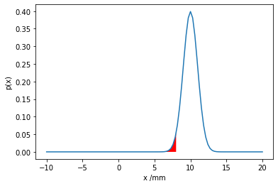
The amount of rainfall in mm on a particular day is given by the normal random variable \(p(x) = \mathcal{N}(\mu=10,\sigma=1)\)
What is the probability of less than 8mm of rainfall?
The probability of less than a certain amount of rainfall is obtained by integrating the probability density function up to that amount. This is equivalent to the cumulative density function at that value.
\(P(\text{rainfall}<8mm) = \int_{-\infty}^{8mm} p(x) dx = F(x=8mm)\)
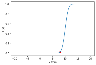
In the following code snippet we evaluate the CDF of the random variable using scipy.stats.
Then we plot the PDF and CDF of the random variable using matplotlib and show the relevant integrated area of the random variable in red.
import matplotlib.pyplot as plt
import scipy.stats
import numpy as np

print(scipy.stats.norm.cdf(8, loc=10, scale=1))


plot_x_range = np.linspace(-10, 20, 100)
plot_x_range_integrate = np.linspace(-10, 8, 100)
plt.plot(plot_x_range, scipy.stats.norm.pdf(plot_x_range, loc=10, scale=1))
plt.fill_between(
    plot_x_range_integrate,
    0,
    scipy.stats.norm.pdf(plot_x_range_integrate, loc=10, scale=1),
    facecolor="red"
)
plt.xlabel("x /mm")
plt.ylabel("p(x)")
plt.show()

plot_x_range = np.linspace(-10, 20, 100)
plt.plot(plot_x_range, scipy.stats.norm.cdf(plot_x_range, loc=10, scale=1))
plt.scatter(8, scipy.stats.norm.cdf(8, loc=10, scale=1), color='red')
plt.xlabel("x /mm")
plt.ylabel("F(x)")
plt.show()
0.022750131948179195
Do you notice anything strange about this model? The probability of a negative amount of rainfall is small, but non-zero. Can you think of a way to change the support of the probability distribution and thereby improve the model?
Worked example : elementary probability theory
Consider two events: a patient having a disease \(A_P\), and the patient testing positive for the disease \(A_T\). The two events are associated with the probabilities \(P(A_P)=0.001\) for the patient having the disease, \(P(A_T)=0.1\) for a random patient testing positive and \(P(A_T|A_P)=x\) for the patient testing positive if they have the disease. Plot the probability that a patient has the disease if they test posititive, \(P(A_P|A_T)\), as a function of \(x\):
We know \(P(A_P|A_T)=\frac{P(A_P\cap A_T)}{P(A_T)} = \frac{P(A_T|A_P) P(A_P)}{P(A_T)}\)
prob_infected = 0.001
prob_positive_test = 0.1


def prob_true_positive(x): return x * prob_infected / prob_positive_test


plot_x_range = np.linspace(0, 1, 10)
plt.plot(plot_x_range, prob_true_positive(plot_x_range))
plt.xlabel("$P(A_T|A_P)$")
plt.ylabel("$P(A_P|A_T)$")
plt.show()
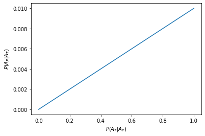
So even with a perfect test, \(P(A_T|A_P)=1\), the probability of having the disease after testing positive is only 0.01. This makes sense because very few people have the disease but the probability of the test being positive is much higher, i.e. 0.1 >> 0.001
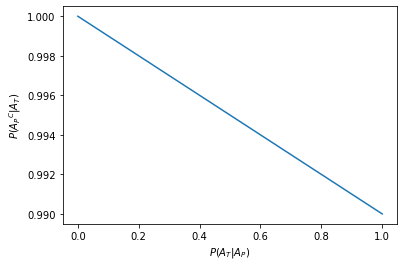
This is clear when we plot the number of false positives, \(P({A_P}^C|A_T) = 1-P({A_P}|A_T)\)
plt.plot(plot_x_range, 1 - prob_true_positive(plot_x_range))
plt.xlabel("$P(A_T|A_P)$")
plt.ylabel("$P({A_P}^C|A_T)$")
plt.show()
Computation with Probabilistic Models
The expectation (mean value) of a general function \(g(x)\) with respect to an uncertain variable, which is modelled with a probability distribution \(p(x)\), can be evaluated as
where we now allow \(x\) to have multiple components.
In the most general case, one can draw realisations, known as samples, from the random variable by selecting values for the variable in the ratio of their assigned probability densities. Given \(M\) samples drawn from \(p(x)\), \(\{ x_{(1)}, \ldots, x_{(M)} \}\), \(\operatorname{\mathbb{E}}[g(X)]\) can be approximated by the Monte Carlo estimator
The error of the Monte Carlo estimator is given by
where \(\sigma_g^2\) is the unbiased sample estimator of the variance of \(g\) [33]. Clearly the error in the estimator decreases with \(\frac{1}{\sqrt{M}}\), so collecting more samples will slowly decrease the error in the estimator [34]. However in many circumstances collecting more samples of \(M\) is not feasible, and \(\sigma_g\) may be large.
Therefore, in practice, more efficient methods are used to compute the expectation. In Reliability Analysis efficient methods for solving a specific form of this integral from engineering reliability analysis will be explained. However, it is useful to note there are some more general efficient approaches for computing an approximation of the expectation in (1).
For example, provided that \(g(x)\) can be differentiated, one can attempt to approximate the expectation in (1) with a Taylor expansion
where \(\mu_X\) is the mean of random variable \(X\). When \(g(x)\) is linear, the the expectation in (1) can therefore be calculated trivially, since \(X - \mu_X = 0\) and \(g''(x) = 0\). If \(g(x)\) is non-linear then using the approximation \(\operatorname{\mathbb{E}}[g(X)] \approx \operatorname{\mathbb{E}} [g(\mu_X)]\) is correct only to first order [35]. At the expense of generality, the expectation is evaluated using only two evaluations of \(g(x)\), which is a clear advantage when \(g(x)\) is expensive to evaluate, or the computation of \(\operatorname{\mathbb{E}}[g(X)]\) is required quickly. This idea is applied to engineering in the Kalman Filter and Extended Kalman Filter [35].
[36] proposed a more accurate approximate method for approximating the expectation in (1) which requires few evaluations of \(g(x)\), and does not require \(g(x)\) to be differentiated. The Unscented Transformation, sometimes referred to as deterministic sampling, requires the computation of so called sigma points which are specially chosen represent the covariance of the input distributions. It is then only required to compute \(g(x)\) for these sigma points, after which a weighted average is used to obtain the approximation of the expectation in (1). [35] demonstrate that the Unscented Transformation is accurate to at least second order, but potentially to third or forth order in some cases. The number of sigma points required, and hence the cost of the computation, depends linearly on the dimensionality of \(x\). Although this approach is more generally applicable and accurate than the Taylor Series method, the Unscented Transformation is limited to use cases where \(x\) has reasonably low dimensionality, because otherwise too many evaluations of \(g(x)\) are required. The method has been applied to engineering in the Unscented filter [35] and uncertainty quantification in the nuclear industry by [37] and [38].
In order to avoid these approximations, techniques can be used to obtain more accurate approximations of \(g(x)\) in specific cases (metamodels), or alternatively efficient sampling strategies can be used. This is discussed in Reliability Analysis for application to reliability analysis.
Worked example : Computation with a probabilistic model
Again, the amount of rainfall in mm on a particular day is given by the normal random variable \(p(x) = \mathcal{N}(\mu=10,\sigma=1)\). It is known that the number of umbrellas sold in London on a particular day is given by \(g(x) = 1000 x^2\).
Estimate the number of umbrellas sold in London given our uncertain model of rainfall.
Analytically evaluating this integral in a popular computer algebra system yields \(\text{Umbrellas sold}=101000\).
# First try Monte Carlo integration
n_samples = 100
samples_x = scipy.stats.norm(loc=10, scale=1).rvs(n_samples)


def g(x): return 1000 * x ** 2


umbrellas_sold = np.mean(g(samples_x))

print("We expect that {} umbrellas were sold".format(umbrellas_sold))

error = np.std(g(samples_x)) / np.sqrt(n_samples-1)

print("The error of this Monte Carlo estimator is {}".format(error))
We expect that 101287.30984936524 umbrellas were sold
The error of this Monte Carlo estimator is 2063.720321793903
Using {} in a string with .format() is a compact and readable method of inserting a quantity into a print statement. The scipy stats library is used for the random variables, and the expectation is taken using np.mean.
Note that we divide the standard deviation from numpy by \(M-1\), since the output of np.std is the standard deviation and not the unbiased estimator for sample standard deviation.
Most importantly the Monte Carlo simulation agrees with the analytic result!
We can plot how the result changes with an increasing number of samples.
def monte_carlo_simulation(n_samples):
    """
    Monte Carlo Simulation for number of umbrellas sold in London on a
      particular day
        Args:
            n_samples (int): Number of samples to be made in Monte Carlo
              simulation
        Returns:
            Number of umbrellas sold (float): The expected number of umbrellas
              sold
            error (float): The error in the estimated number of umbrellas sold
    """
    samples_x = scipy.stats.norm(loc=10, scale=1).rvs(n_samples)
    def g(x): return 1000 * x ** 2

    umbrellas_sold = np.mean(g(samples_x))

    error = np.std(g(samples_x)) / np.sqrt(n_samples-1)
    return umbrellas_sold, error


number_of_samples = [10, 20, 30, 40, 50, 100, 200, 1000, 10000, 100000]
simulation_results = [monte_carlo_simulation(n) for n in number_of_samples]

plt.plot(number_of_samples, list(zip(*simulation_results))[0])
plt.plot([0, 100000], [101000]*2)
plt.errorbar(number_of_samples, *zip(*simulation_results))
plt.xlabel("Number of samples")
plt.ylabel("Umbrellas sold")
plt.xscale("log")
plt.show()
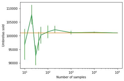
Notice that all simulation results are within 3 standard deviations of the true value.
The true value from the analytic calculation is shown with an orange line. The simulation results and error bars are shown in green.
Note that we used several useful features of python in the above code.
We use a docstring below the function definition to explain what the purpose of the function is and the expected inputs and outputs.
Note that the defined function returns two outputs - these are treated like a tuple object when inserted into the list. zip(*simulation_results) converts the list of tuples into a tuple of lists.
As in the previous example, the sampling is vectorised (i.e. no loop is used in generating the samples for each simulation) to reduce the time required for computation.
A list comprehension is used to tidily obtain the results from the Monte Carlo simulation and put these into a list.
To reduce the number of samples required we now evaluate the integral using a Taylor Series.
def g(x): return 1000 * x ** 2


def g_dash_dash(x): return 1000 * 2


loc = 10
scale = 1

zero_order_taylor_series = g(loc)
# first order contribution is zero!
second_order_term = g_dash_dash(loc) * 0.5 * scale
taylor_series_umbrellas = zero_order_taylor_series + second_order_term

print("Taylor series - umbrellas sold: {}".format(taylor_series_umbrellas))
Taylor series - umbrellas sold: 101000.0
The correct result is obtained exactly! This is because the third and higher derivatives of \(g(x)\) are zero!