Learning bounds on a model
Instead of learning a probability distribution to describe the effect of one variable on another, one may instead attempt to learn a function which maps the input variables to an interval representing the possible range of the output. Such models are known as interval predictor models. Sometimes the predicted intervals have an associated confidence level (or a bound on the confidence level), and as such they can be considered as bounds on the quantiles of a random variable [55]. Typically the obtained intervals represent an outer approximation, i.e. the intervals are overly wide and hence conservative in an engineering sense. An interval predictor model can be seen as prescribing the support of a Random Predictor Model, which is defined as a function which maps input variables to an output random variable. A Gaussian Process Model is a specific case of a Random Predictor Model.
In this section, we describe how interval predictor models can be trained in practice. We then describe how the theory of scenario optimisation can be used to provide guaranteed bounds on the reliability of the trained interval predictor models, for the purpose of validation.
Training interval predictor models
Let us consider a black box model (sometimes referred to as the Data Generating Mechanism or DGM) which acts on a vector of input variables \(x \in \mathbb{R}^{n_x}\) to produce an output \(y \in \mathbb{R}\). We wish to obtain the two functions \(\overline{y}(x)\) and \(\underline{y}(x)\) which enclose a fraction, \(\epsilon\), of samples from the DGM, i.e. samples of \(y(x)\) where \(x\) is sampled from some unknown probability density. The functions \(\overline{y}(x)\) and \(\underline{y}(x)\) are bounds on a prediction interval, and as such we wish them to be as tight as possible. This can be written as a so-called chance constrained optimisation program: \(\operatorname{argmin}_{\boldsymbol{p}}{\{\mathbb{E}_x(\overline{y}_{\boldsymbol{p}}(x) - \underline{y}_{\boldsymbol{p}}(x)) : P\{\overline{y}_{\boldsymbol{p}}(x) > y(x) > \underline{y}_{\boldsymbol{p}}(x) \} \le \epsilon\}},\) where \(\boldsymbol{p}\) is a vector of function parameters to be identified, and \(\epsilon\) is a parameter which constrains how often the constraints may be violated. Chance constrained optimisation programs can be solved by using a so-called scenario program, where the chance constraint is replaced with multiple sampled constraints based on data, i.e.
where \(\mathcal{X}_\text{train} = \{ \{x^{(1)}, y^{(1)}\}, ..., \{x^{(n)}, y^{(n)}\} \}\) are sampled from the DGM. Most of the literature on scenario optimisation Theory aims to obtain bounds on \(\epsilon\). Finding bounds on \(\epsilon\) using scenario optimisation is easier in practice than other similar methods in statistical learning theory, since no knowledge of the Vapnik-Chervonenkis dimension (a measure of the capacity of the model, which is difficult to determine exactly) is required.
A key advantage over other machine learning techniques is that interval training data (i.e. where the training data inputs are given in the form \(x^{(i)} \in [\underline{x}^{(i)}, \overline{x}^{(i)}]\) due to epistemic uncertainty or some other reason) fits into the scenario optimisation framework coherently [56]. This can be seen as equivalent to defending against the attack model of adversarial examples considered by [57], where the network is trained to produce the same outputs for small perturbations of the input data. The framework also permits robustness against uncertainty in training outputs, i.e. \(y^{(i)} \in [\underline{y}^{(i)}, \overline{y}^{(i)}]\), where \(y^{(i)}\) is a single training example output.
Convex interval predictor models
If the objective and constraints for the scenario program are convex then the program can be easily solved, and bounds can be put on \(\epsilon\). We will approximate the DGM with an interval predictor model (IPM) which returns an interval for each vector \(x\in X\), the set of inputs, given by
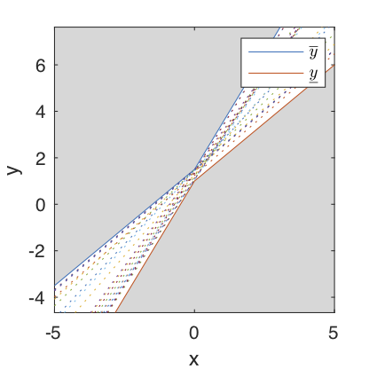
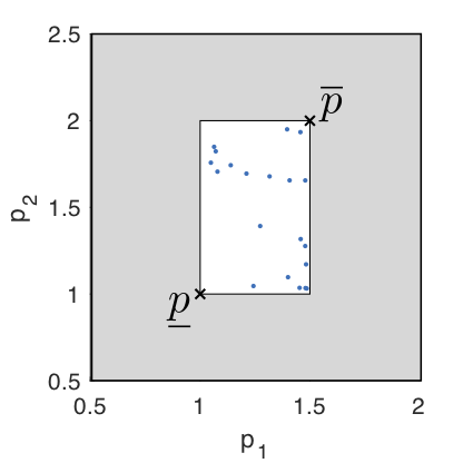
where \(G\) is an arbitrary function and \(\boldsymbol{p}\) is a parameter vector. By making an approximation for \(G\) and considering a linear parameter dependency (12) becomes \(I_y(x,P)=\big\{ y=\boldsymbol{p}^{T} \phi (x),\boldsymbol{p} \in P \big\} ,\) where \(\phi (x)\) is a basis (polynomial and radial bases are commonly used), and \(\boldsymbol{p}\) is a member of a convex parameter set. The convex parameter set is usually assumed to be either ellipsoidal or hyper-rectangular [58]. [59] demonstrates that hyper-rectangular parameters sets result in an IPM with bounds with a convenient analytical form. The hyper-rectangular parameter uncertainty set can be defined as \(P=\big\{\boldsymbol{p}:\underline{\boldsymbol{p}} \leq \boldsymbol{p} \leq \overline{\boldsymbol{p}} \big\},\) where \(\underline{\boldsymbol{p}}\) and \(\overline{\boldsymbol{p}}\) are parameter vectors specifying the defining vertices of the hyper rectangular uncertainty set. The IPM with linear parameter dependency on the hyper-rectangular uncertain set of parameters is defined by the interval \(I_y(x,P)=[\underline{y}(x,\overline{\boldsymbol{p}},\underline{\boldsymbol{p}}),\overline{y}(x,\overline{\boldsymbol{p}},\underline{\boldsymbol{p}})],\) where \(\underline{y}\) and \(\overline{y}\) are the lower and upper bounds of the IPM, respectively. Explicitly, the lower bound is given by \(\underline{y}(x,\overline{\boldsymbol{p}},\underline{\boldsymbol{p}}) = \overline{\boldsymbol{p}} ^T \left( \frac{\phi(x)-|\phi(x)|}{2} \right)+\underline{\boldsymbol{p}} ^T \left( \frac{\phi(x)+|\phi(x)|}{2} \right),\) and the upper bound is given by \(\overline{y}(x,\overline{\boldsymbol{p}},\underline{\boldsymbol{p}}) = \overline{\boldsymbol{p}} ^T \left( \frac{\phi(x)+|\phi(x)|}{2} \right)+\underline{\boldsymbol{p}} ^T \left( \frac{\phi(x)-|\phi(x)|}{2} \right).\) To identify the hyper-rectangular uncertainty set one trains the IPM by minimising the value of \(\delta_y(x,\overline{\boldsymbol{p}},\underline{\boldsymbol{p}})=(\overline{\boldsymbol{p}}-\underline{\boldsymbol{p}})^T |\phi (x) |,\) subject to the constraint that the training data points fall inside the bounds on the IPM, by solving the linear and convex optimisation problem
The constraints ensure that all data points to be fitted lie within the bounds and that the upper bound is greater than the lower bound. This combination of objective function and constraints is linear and convex [59]. In this thesis all interval predictor models have polynomial bases, i.e. \(\phi(x)=\left[1,x^{i_2},x^{i_3},...\right]\) with \(x=[x_a,x_b,...]\) and \(i_j=[i_{j,a},i_{j,b},...]\) with \(i_j\ne i_k\) for \(j\ne k\).
For illustrative purposes an example degree 2 IPM is shown without training data points in Fig. 3. The hyper rectangular uncertainty set corresponding to the IPM in Fig. 3 is plotted in Fig. 4. The discontinuity observed in the upper and lower bounds is a consequence of the chosen basis, and can be avoided by choosing a basis where \(\phi(x)=|\phi(x)|\).
Non-convex interval predictor models
In some circumstances engineers may wish to represent more complex functions with IPMs, and hence the functions used to represent the bounds of the IPM may have more trainable parameters. The interior point method used to solve linear optimisation programs, such as those used for convex IPMs, has complexity \(d^2 n_\text{cons}\), where \(d\) represents the number of optimisation variables and \(n_\text{cons}\) represents the number of constraints in the optimisation (which in this case scales linearly with the number of training data points), and hence the method does not scale well to IPMs with large numbers of trainable parameters [45].
Neural networks enable uncertainty models to be created with vast numbers of parameters in a feasible computational time. Neural networks with interval outputs were proposed by [60], and further described by [61]. In these papers the learning takes place by identifying the weights \(W\), which solve the following program:
where \(\overline{y}(x)\) and \(\underline{y}(x)\) are obtained from two independent neural networks, such that \(\overline{y}(x)\) and \(\underline{y}(x)\) are the output layers of networks, such as those defined by (9). In practice this problem is solved by using a mean squared error loss function with a simple penalty function to model the constraints. In general, penalty methods require careful choice of hyper-parameters to guarantee convergence. These neural networks act in a similar way to interval predictor models, however the interval neural networks do not attempt to use the training data set to bound \(\epsilon\). [62] define similar networks with fuzzy parameters to operate on fuzzy data. The fuzzy neural networks are trained by minimising a least square loss function (a set inclusion constraint is not used), which can also be applied to time series data sets. These approaches are very different from the approach of [63], where a traditional neural network loss function is intervalised using interval arithmetic.
[64] extended the scenario approach to non-convex optimisation programs, and hence applied the approach to a single layer neural network, with a constant width interval prediction, which was trained using the interior-point algorithm in Matlab. In other words the following program is solved:
where \(h\) is a real number, and \(\hat{y}\) represents the central line of the prediction obtained from the same network specified by (9). The bounds on the prediction interval are therefore given by \(\overline{y}(x) = \hat{y}(x) + h\) and \(\underline{y}(x) = \hat{y}(x) - h\). The constant width interval neural network expresses homoscedastic uncertainty. The solution to the optimisation program in (15) can also be obtained by finding the neural network weights which minimise the so-called maximum-error loss:
where \(h\) is the minimum value of the loss. It is trivial to show this is true, since the set inclusion constraint in (15) requires that \(h\) is larger than the absolute error for each data point in the training set [65].
In [66] a back propagation algorithm for Neural Networks with interval predictions is proposed. A modified maximum-error loss is used. The approach can accommodate incertitude in the training data. A key result is that, by using minibatches, the complexity of the proposed approach does not directly depend upon the number of training data points as with other Interval Predictor Model methods.
Validating models with the scenario approach
We will first present an overview of the scenario optimisation theory for the validation of models in the convex case, before describing more general techniques which apply in the non-convex case.
Convex case
Intuition tells us that the solution of the scenario program will be most accurate when the dimensionality of the design variable is low and we take as many samples of the constraints as possible (in fact, an infinite number of sampled constraints would allow us to reliably estimate \(P\{\overline{y}_{\boldsymbol{p}}(x) > y(x) > \underline{y}_{\boldsymbol{p}}(x) \}\), and hence solve the program exactly). However, in practice obtaining these samples is often an expensive process. Fortunately, the theory of scenario optimisation provides robust bounds on the robustness of the obtained solution. The bounds generally take the following form: \(P^n(V(\hat{z}_n)>\epsilon)\le\beta.\) This equation states that the probability of observing a bad set of data (i.e. a bad set of constraints) in future, such that our solution violates a proportion greater than \(\epsilon\) of the constraints (i.e. \(V(\hat{z}_n)>\epsilon\) where \(V(\hat{z}_n) = \frac{1}{n} \sum_i^n {V^{(i)}}\) and \(V^{(i)} = 1\) only if \(\overline{y}_{\boldsymbol{p}}(x) > y(x) > \underline{y}_{\boldsymbol{p}}(x)\)), is no greater than \(\beta\). The scenario approach gives a simple analytic form for the connection between \(\epsilon\) and \(\beta\) in the case that the optimisation program is convex:
where \(n\) is the number of constraint samples in the training data set used to solve the scenario program, and \(d\) is the dimensionality of the design variable, \(z\). For a fixed \(d\) and \(n\) we obtain a confidence-reliability relationship: by decreasing \(\epsilon\) slightly, \(1-\beta\) can be made to be insignificantly small. Other tighter bounds exist in the more recent scenario optimisation literature, e.g. [67] [68] [69], for example
Crucially the assessment of \(V(\hat{z}_n)\) is possible a priori, although other techniques exist [70]. [71] analyse the reliability of solutions of the maximum error loss functions ((16)) in the scenario framework when \(\hat{y}(x)\) is convex in \(x\) and the function weights.
In the convex case, the a priori assessment is made possible by the fact that the number of support constraints (the number of constraints which if removed result in a more optimal solution) for a convex program is always bounded by the dimensionality of the design variable. [72] explore this connection for convex programs in further detail, by analysing the number of support constraints after a solution is obtained. In fact, the bound in (18) if often overly conservative, because in many cases the number of support constraints is less than the dimensionality of the design variable, and hence a more accurate bound on the reliability of the IPM can be obtained. The improved bound is given by letting \(\epsilon\) be a function of the number of support constraints \(s^*_n\) such that \(\epsilon(s^*_n)=1-t(s^*_n)\). Then for \(0<\beta<1\) and \(0<s^*_n<d\) the equation
has one solution, \(t(k)\) in the interval \([0,1]\).
This idea has a deep connection with the concept of regularisation in machine learning [73]. [74] demonstrates how the number of support constraints of a scenario program can be used to iteratively increase the number of sampled constraints, which requires fewer sampled constraints in total than (18) for equivalent \(\epsilon\) and \(\beta\). For a non-convex program, the number of support constraints is not necessarily less than the dimensionality of the design variable, and therefore a new approach is required, which we describe in the following section.
Non-convex case
[75] provide the following bound for the non-convex case: \(P^n(V(\hat{z}_n)>\epsilon(s))<\beta,\) where
and \(s\) is the cardinality of the support set (in other words, the number of support constraints). The behaviour of this bound is similar to the convex case since in general increasing \(n\) should increase the size of the support set.
Finding the cardinality of the support set is in general a computationally expensive task, since the scenario program must be solved \(n\) times. [64] present a time-efficient algorithm which only requires that the scenario problem is solved \(s\) times.
A posteriori frequentist analysis
When data is available in abundance, as is typically the case in most machine learning tasks where a neural network is currently used, \(V(\hat{z}_n)\) can be evaluated more easily by using a test set to collect samples from \(V(\hat{z}_n)\). Estimating \(V(\hat{z}_n)\) is similar to estimating a probability of failure in the well known reliability theory. Therefore one can construct a Monte Carlo estimator of \(V(\hat{z}_n)\), or use more advanced techniques from reliability analysis if it is possible to interact with the data generating mechanism. For example, if the number of test data points is large we can use the normal approximation Monte Carlo estimator of \(V(\hat{z}_n)\) with \(V(\hat{z}_n)\approx \frac{N_v}{N_t}\) and standard deviation \(\sqrt{\frac{\frac{N_v}{N_t}(1-\frac{N_v}{N_t})}{N_t}}\), on a test set of size \(N_t\), where \(N_v\) data points fall outside the interval bounds of the neural network.
A particularly robust method of estimating the probability of a binary outcome involves using the binomial confidence bounds. In this case specifically, one can bound \(V(\hat{z}_n)\) with the desired confidence using the binomial confidence bounds: \(\sum_{i=0}^{N_t-N_v}\binom{N_t}{i}(1-\underline{v})^i\underline{v}^{N_t-i}=\frac{\beta}{2}\) and \(\sum_{i=N_t-N_v}^{N_t}\binom{N_t}{i}(1-\overline{v})^i\overline{v}^{N_t-i}=\frac{\beta}{2},\) where \(P(V(\hat{z}_n)<\overline{v} \cap V(\hat{z}_n)>\underline{v})=\beta\). Estimating \(V(\hat{z}_n)\) using a test set also offers the advantage that when the neural network is used for predictions on a different data set, \(V(\hat{z}_n)\) can be evaluated easily. If the value of \(V(\hat{z}_n)\) obtained on the test set is higher than that on the training dataset, one can apply regularisation in order to implicitly reduce the size of the support set and increase \(V(\hat{z}_n)\) on the test set (e.g. dropout regularisation, or \(\ell_2\) regularisation on the weights).
This methodology is ideal for models with a complex training scheme, where determining the support set would be prohibitively expensive. Note that the probabilistic assessment of the reliability of the model takes place separately from the training of the regression model, such that it is still robust, even if there is a problem with the regression model training. This is an important advantage over Variational Inference methods which are often used with neural networks.
Software for interval predictor models
[76] describe the first open source software implementation of interval predictor models in the generalised uncertainty quantification software OpenCossan, which is written in Matlab. The OpenCossan software allows convex IPMs to be trained, with hyper-rectangular uncertainty sets. The OpenCossan software is modular and allows the IPMs to be automatically trained as approximations of expensive engineering models, and then used in other engineering calculations, e.g. design optimisation. A partial Python port of the OpenCossan IPM code was released as open source software by [77].
The introduced software has been applied in [78], to study fatigue damage estimation of offshore wind turbines jacket substructure.
Worked example : linear regression
We repeat the previous linear regression example using the PyIPM Interval Predictor Model library.
Since the IPM makes fewer assumptions than the parametric model we will require more data to learn an effective model.
Therefore we will generate training data from a toy function \(1000 x^2 + \epsilon\), where \(\epsilon\) is randomly distributed noise with standard deviation \(20000\).
import PyIPM
import numpy as np
import matplotlib.pyplot as plt

rainfall = 13 * np.random.rand(100).reshape(-1, 1)
umbrellas = 1000 * rainfall.squeeze(-1) ** 2 + 20000 * np.random.rand(100)

model = PyIPM.IPM(polynomial_degree=2)

model.fit(rainfall, umbrellas)

x_plot = np.arange(0, 13, 0.1)
upper_bound, lower_bound = model.predict(x_plot.reshape(-1, 1))

plt.scatter(rainfall, umbrellas, label="Training Data")
plt.fill_between(
    x_plot,
    lower_bound.squeeze(-1),
    upper_bound.squeeze(-1),
    alpha=0.3,
    label="IPM"
)
plt.legend()
plt.show()

print("For a test set generated from the same function as the training data, "
      "our model predictions will be enclose the test set with probability "
      "greater than {}".format(model.get_model_reliability()))
     pcost       dcost       gap    pres   dres   k/t
 0: -2.3064e-11 -1.4903e-10  2e+06  1e-01  1e+02  1e+00
 1:  2.0572e+04  2.1734e+04  3e+05  1e-02  1e+01  1e+03
 2:  1.9839e+04  1.9904e+04  2e+04  1e-03  1e+00  6e+01
 3:  1.9085e+04  1.9106e+04  5e+03  3e-04  2e-01  2e+01
 4:  1.9057e+04  1.9067e+04  2e+03  1e-04  1e-01  9e+00
 5:  1.9026e+04  1.9027e+04  2e+02  1e-05  1e-02  1e+00
 6:  1.9021e+04  1.9021e+04  2e+01  2e-06  1e-03  1e-01
 7:  1.9020e+04  1.9020e+04  5e-01  3e-08  2e-05  2e-03
 8:  1.9020e+04  1.9020e+04  5e-03  3e-10  2e-07  2e-05
 9:  1.9020e+04  1.9020e+04  5e-05  3e-12  2e-09  2e-07
Optimal solution found.
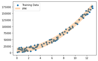
For a test set generated from the same function as the training data, our model predictions will be enclose the test set with probability greater than 0.7704137287382764
This example demonstrates the benefits of Interval Predictor Models: few assumptions are required, but a model which fits the data well can be obtained, alongside rigorous uncertainty quantification.