Reliability analysis with probability boxes
Problem definition
Probability boxes offer a hybrid of the convex set and probabilistic approaches for reliability analysis. In structural reliability analysis with probability boxes, the objective is to compute the failure probability in the same sense as with traditional random variables in Reliability theory. However, it is now impossible to compute an exact value for the failure probability; only bounds on the failure probability are available [99]. For distributional probability boxes, \(f_{X_{\boldsymbol{\theta}}}({\boldsymbol{x}})\) for \(\boldsymbol{\theta} \in \Theta\), the bounds on the failure probability can be found by solving the integrals
and
For distribution-free probability boxes given by \([\underline{F}_i(x_i), \overline{F}_i(x_i)]\), each system variable can be written as a function of separate probabilistic and set based variables as \(x_i' = \underline{F}_i^{-1}(\alpha_i) + (\overline{F}_i^{-1}(\alpha_i)-\underline{F}_i^{-1}(\alpha_i)){\theta}_i\), where the aleatory variable \(\alpha=(\alpha_1,\alpha_2,\ldots)\) is a uniformly distributed random vector with the same dimensionality as \(\boldsymbol{x}\), and \(\boldsymbol{\theta} \in \Theta\) is the unit hyper-cube with the same dimensionality as \(\boldsymbol{x}\) [26]. This enables the performance function \(g(\boldsymbol{x})\) to be rewritten in terms of \(\boldsymbol{\alpha}\) and \(\boldsymbol{\theta}\), i.e. \(g(\boldsymbol{\alpha}, \boldsymbol{\theta})\). Bounds on the failure probability can then be obtained by evaluating
and
where the upper and lower performance function are obtained from \(\underline{g}(\boldsymbol{\alpha}) = \min_{\boldsymbol{\theta} \in \Theta} g(\boldsymbol{\alpha}, \boldsymbol{\theta})\) and \(\overline{g}(\boldsymbol{\alpha}) = \max_{\boldsymbol{\theta} \in \Theta} g(\boldsymbol{\alpha}, \boldsymbol{\theta})\)
By finding the envelope of a distributional probability box, the algorithm for computing the failure probability for the distribution-free case can be applied. As expected, [100] demonstrate that this results in overly conservative bounds on the failure probability, since clearly information is lost by taking the envelope of the distributional probability box. Therefore, only (30) and (31) should be applied when computing failure probabilities with distributional probability boxes.
Methods to compute the failure probability
In this section we concentrate on methods to compute the failure probability for distributional probability boxes.
Monte Carlo estimators
A Monte Carlo estimator can be applied for the integrals in the failure probability computation with distribution-free probability boxes ((30) and (31) to yield the bounds \([\underline{P}_f, \overline{P}_f] = [\min_{\boldsymbol{\theta} \in \Theta} \frac{1}{N} \sum_{i=1}^{N} \mathbb{I}_f({\boldsymbol{x}^{(i)}_{\boldsymbol{\theta}}}), \max_{\boldsymbol{\theta} \in \Theta} \frac{1}{N} \sum_{i=1}^{N} \mathbb{I}_f({\boldsymbol{x}^{(i)}_{\boldsymbol{\theta}}})],\) where the samples \(\boldsymbol{x}^{(i)}_{\boldsymbol{\theta}}\) are drawn from \(f_{X_{\boldsymbol{\theta}}}({\boldsymbol{x}})\). This is the double loop Monte Carlo approach; an inner loop is used to compute a Monte Carlo estimator which is optimised over in the outer loop [28]. The outer loop optimisation can be evaluated using brute force grid sampling of \(\boldsymbol{\theta}\), which is known as naïve double loop Monte Carlo simulation. It is usually more efficient to use an efficient global optimisation algorithm to evaluate the optimisation loop, such as Bayesian Optimisation, or a genetic algorithm [26].
Evaluating the failure probability using double loop Monte Carlo simulation is computationally expensive, since now each inner loop Monte Carlo estimator must be computed multiple times. This is particularly the case when the problem dimensionality is large or the failure probability is small. [29] shows that the bias of the estimator is negative, and the magnitude of the bias decreases as more samples are made.
Imprecise First Order Reliability Method
A generalisation of FORM for systems with components which are described by probability boxes was introduced by [101]. The system’s performance function must be written in the load resistance form ((22)), and the system must have one strength and one load component. Therefore, the system variables consist of the resistance variable with mean \(\mu_R\in[\underline{\mu_R}, \overline{\mu_R}]\) and standard deviation \(\sigma_R\in[\underline{\sigma_R}, \overline{\sigma_R}]\), and load variable with mean \(\mu_L\in[\underline{\mu_L}, \overline{\mu_L}]\) and standard deviation \(\sigma_L\in[\underline{\sigma_L}, \overline{\sigma_L}]\). Then the failure probability lies in the interval \([\underline{P}_f,\overline{P}_f]=[\phi(-\overline{\beta}), \phi(-\underline{\beta})]\), where \(\overline{\beta}=\frac{\overline{\mu}_R-\underline{\mu_L}}{\underline{\sigma_L}^2+\underline{\sigma_R}^2},\) and \(\underline{\beta}=\frac{\underline{\mu}_R-\overline{\mu}_L}{\overline{\sigma}_L^2+\overline{\sigma}_R^2}.\)
In more complex cases, one may need to solve an optimisation program to find the reliability index [102]. For example, one could imagine a system which fails if the sum of many different products of probability box distributed variables falls below a threshold.
Line sampling
[26] describes two ways in which Line Sampling can be used to increase the efficiency of probability box propagation. Line Sampling can be applied as an alternative to the Monte Carlo estimator used to approximate the integral in the double loop approach ((30) and (31)). Alternatively, Line Sampling can be applied to the aleatory variables \(\boldsymbol{\alpha}\) for the upper and lower performance functions in (32) and (33). When Line Sampling is applied in the aleatory space, the importance direction updating strategy proposed by [26] significantly increases the accuracy of the computation. Judged by number of samples required for computation, Line Sampling is close to the state of the art. However, Line Sampling is ineffective on highly non-linear limit state surfaces.
Importance sampling
The Importance Sampling estimator in (28) can be applied to greatly reduce the number of samples required when computing the failure probability for a system subject to probability box random variables [100]. The bounds on the failure probability are given by \(\underline{P}_f=\min_{\boldsymbol{\theta} \in \Theta}{\int \mathbb{I}_f(\boldsymbol{x}) \frac{f_{X_{\boldsymbol{\theta}}}({\boldsymbol{x}})}{h(\boldsymbol{x})} h(\boldsymbol{x}) d\boldsymbol{x} } = \min_{\boldsymbol{\theta}} \frac{1}{N} \sum_{i=1}^N \mathbb{I}_f({\boldsymbol{x}}^{(i)}) \frac{f_{X_{\boldsymbol{\theta}}}({{\boldsymbol{x}}^{(i)}})}{h({\boldsymbol{x}}^{(i)})}\) and \(\overline{P}_f=\max_{\boldsymbol{\theta} \in \Theta}{\int \mathbb{I}_f(\boldsymbol{x}) \frac{f_{X_{\boldsymbol{\theta}}}({\boldsymbol{x}})}{h(\boldsymbol{x})} h(\boldsymbol{x}) d\boldsymbol{x} } = \max_{\boldsymbol{\theta}} \frac{1}{N} \sum_{i=1}^N \mathbb{I}_f({\boldsymbol{x}}^{(i)}) \frac{f_{X_{\boldsymbol{\theta}}}({{\boldsymbol{x}}^{(i)}})}{h({\boldsymbol{x}}^{(i)})},\) where the samples \({\boldsymbol{x}}^{(i)}\) are drawn from the proposal distribution \(h(\boldsymbol{x})\). The proposal distribution can be iteratively updated to provide more accurate results. [103] demonstrates that the bias in both cases is negative and decreases in magnitude as more samples are collected. The Importance Sampling estimator requires a similar number of samples to Line Sampling.
Multi level metamodels
Multilevel Metamodelling requires the creation of two Gaussian Process emulators [104]. The first metamodel is created for the performance function in the space of the system variables \(\boldsymbol{x}\), using Adaptive Kriging Monte Carlo simulation. The second metamodel is used to perform Bayesian Optimisation on the obtained failure probability from the first metamodel, in the epistemic space. This greatly reduces the amount of repeated similar evaluations of the system model, and hence the Multi-level metamodelling technique is close to state of the art when judged by number of required samples.
Interval Predictor Models
[105] uses an IPM as a metamodel to propagate probability boxes. In the first two algorithms, the performance function is modelled as a function with unknown noise structure in the aleatory space and supplemented by a modified performance function. In the third algorithm, an Interval Predictor Model is constructed and a re-weighting strategy used to find bounds on the probability of failure.