Reliability analysis with random variables
Problem definition
Reliability theory
The aim of structural reliability analysis is to compute the probability that the performance of a system is less than some specified threshold; this probability is known as the failure probability of the system. Firstly, the performance of the system, \(g({\boldsymbol{x}})\), is defined as a function of the vector of system variables, \(\boldsymbol{x} = (x_1, x_2,\ldots,x_i,\ldots)\). The performance function is negative when the system fails, and otherwise positive. Then the failure probability can be found by solving the integral
where the indicator function, \(\mathbb{I}_f({\boldsymbol{x}})\), is defined as \(\mathbb{I}_f({\boldsymbol{x}}) = \left\{\begin{array}{lr} 1, & \text{for } g({\boldsymbol{x}})<0\\ 0, & \text{for } g({\boldsymbol{x}})\ge0 \end{array}\right\} ,\) and the probability density function of the system random variables is \(f_X({\boldsymbol{x}})\) [106]. It is common for the performance function to be defined in the load resistance form, e.g.
where \(R\) are indices corresponding to resistance factors and \(L\) are indices corresponding to load factors, so that the system fails when the sum of loads is greater than the sum of resistances [107]. When the resistance and load are balanced, \(g(\boldsymbol{x})=0\) and the system is on the interface of the safety and failure regions. The limit state surface is specified by the \(\boldsymbol{x}\) for which \(g(\boldsymbol{x})=0\).
In fault tree analysis the failure event of a system is written in terms of failure events for smaller subsystems or components, using Boolean algebra. Probability arithmetic can be used with the fault tree to combine failure probabilities for individual subsystems to obtain the failure probability for the whole system. This requires knowledge of the dependencies between the probability of failure events for the considered sub-systems [106].
Reliability based design optimisation
In reliability based design optimisation (RBDO), a cost function, e.g. the weight or construction cost of the system, is minimised subject to the constraint that the failure probability of the system does not fall below a certain value. The reliability based design optimisation problem can be stated as the optimisation program
where \(\boldsymbol{d}\) is the vector of design variables, \(\text{cost}(\boldsymbol{d})\) is the cost function of the design, \(P_f(\boldsymbol{d})\) is the failure probability of the design, and \(P_\text{target}\) is the target failure probability. Usually the vector of design variables, \(\boldsymbol{d}\), will be parameters of the random variables, \(f_X({\boldsymbol{x}})\), associated with the resistance, such that (23) usually finds a balance between a cost effective design and a design where the resistance of the system is sufficiently greater than the load [106].
In engineering practice the model of the structure is often computationally expensive to evaluate, and therefore it may be more convenient to find a sub-optimal solution to (23), by designing the structure based on engineering judgement. Approximate rules of thumb, such as partial safety factors, allow the reliability of the system to be constrained approximately using analytical equations [106]. Then the full reliability analysis can be performed with the proposed design to ensure that the reliability of the system satisfies the constraints in (23). Hence a safe and efficient design can be obtained with reduced computational effort.
Sensitivity analysis
Sensitivity analysis allows the effect of each uncertain variable on the variability of the model response to be quantified. This can be achieved either by local methods, which describe variability of the model response at the expected value of the system variables, or global methods, which describe the total variability of the model response.
Local sensitivity analysis is often achieved by evaluating the first derivative of the model response with respect to the system variables. Similarly, [108] defines component importance as the partial derivative of the system reliability with respect to the reliability of the component.
Global sensitivity analysis is usually performed by evaluating the Sobol indices,
which describe the contribution of the variance of \(x_i\) to the total variance of the model response \(g(\boldsymbol{x})\), when only \(x_i\) is varied. \(x_{\sim i}\) represents all random variables other than \(x_i\). The Total Effect indices, given by
include the effect of interactions caused by varying \(x_i\) whilst varying other variables [109].
The most simple way to evaluate the Sobol indices and total effect indices is by using a Monte Carlo estimator for the expectation and variance terms in (24) and (25). In some cases, for example when the model has too many parameters or the model is very computationally expensive, it is necessary to use a more complex method to compute the Sobol and total sensitivity indices. For example, the upper bound of the total sensitivity index can be efficiently calculated by integrating the local sensitivity analysis over the whole space of the inputs [110], and the Sobol indices can be efficiently calculated by use of the Fourier Amplitude Sensitivity Testing (FAST) method [111].
Methods to compute the failure probability
In some circumstances the failure probability can be computed analytically, for example when the system variables \(\boldsymbol{x}\) are normally distributed and the performance function is linear [106]. However, often a closed form solution of (21) is not available and hence alternative methods must be used.
Monte Carlo simulation
In general, the failure probability can be computed by Monte Carlo simulation, as discussed for general functions in Models of Uncertainty. The Monte Carlo estimator for the failure probability is
where \(N\) samples, \({\boldsymbol{x}}^{(i)}\), are drawn from the the probability density function of the system random variables \(f_X({\boldsymbol{x}})\). The coefficient of variation of the failure probability estimator is \(\operatorname{CoV}[\hat{P}_f] = \sqrt{\frac{1-P_f}{N P_f}}.\) Therefore, obtaining order of magnitude estimates of \(P_f\) with Monte Carlo simulation requires at least \(\frac{1}{P_f}\) samples, and for an accurate estimate even more samples are required. If \(P_f\) is small and \(g(\boldsymbol{x})\) is expensive to evaluate then the number of samples required is unreasonably large, and more efficient strategies are required to evaluate \(P_f\).
Efficient sampling strategies
Several sampling strategies have been proposed to choose a set of samples which can be used to reduce the variance of the Monte Carlo estimator in (26) without expending additional computational effort. Low-discrepancy sampling strategies aim to choose a set of samples which cover the sampling domain with the desired density. This is often not the case with a small random set of samples, which may fall disproportionately in one area of the sampling domain before the law of large numbers takes effect. Stratified Sampling strategies, such as Latin Hypercube Sampling divide the probability density of the system variables into an \(n\)-dimensional grid, where each grid element contains equal probability density. Then a sample may be chosen at random in each grid element, resulting in a set of samples which covers the sampling domain well. For linear functions it can be shown that this sampling strategy has a lower variance than the traditional Monte Carlo estimator [112]. The main disadvantage of efficient sampling strategies is that the reduction in the coefficient of variation is small when compared to other techniques, e.g. Line Sampling.
First Order Reliability Method
The First Order Reliability Method (FORM) allows the probability of failure of a system to be computed without Monte Carlo simulation. Assuming the system variables are distributed normally and independently, the probability of failure can be obtained analytically if the performance function, \(g(\boldsymbol{x})\), is linear. If the performance function is not linear, a Taylor expansion can be used to find a linear approximation of the limit state function as shown in Fig. 5. If the system random variables are not normally distributed then a transformation must first be applied to the random variables and the limit state function, so that FORM can be applied [106].
The performance function, \(g(\boldsymbol{x})\), is written as the Taylor series expansion
about the point \(\boldsymbol{x}^*\), which is usually chosen to be the point on the limit state surface with the highest probability density. This point is known as the design point, and can be obtained by solving the optimisation program \(\boldsymbol{x}^* = \operatorname{argmin}_{\boldsymbol{x}} \{|\boldsymbol{x}|^2: g(\boldsymbol{x})=0 \}.\) Alternatively, using the assumption of a linear performance function, the design point can be determined using the gradient of the performance function. The reliability index is defined as \(\beta = \sqrt{|\boldsymbol{x}^*|^2}\), and in the case of normally distributed random variables and a linear limit state function \(P_f = \phi(-\beta)\). This can be shown by observing that when \(\boldsymbol{x}^*\) has a standard normal distribution and \(g(\boldsymbol{x})\) is linear (as in (27), the system performance will have a normal distribution with mean \(\mathbb{E}_{\boldsymbol{x}} (g(\boldsymbol{x})) = ( \mathbb{E}_{\boldsymbol{x}} (\boldsymbol{x}) -\boldsymbol{x}^*)\nabla g(\boldsymbol{x}^*) = -\boldsymbol{x}^*\nabla g(\boldsymbol{x}^*)\) and variance \(\operatorname{Var}_{\boldsymbol{x}} (g(\boldsymbol{x})) = |\nabla g(\boldsymbol{x}^*)|^2.\) Therefore, since \(\boldsymbol{x}^* = \beta \frac{\nabla g(\boldsymbol{x}^*)}{\sqrt{ |\nabla g(\boldsymbol{x}^*)|^2}}\), \(P_f = \phi\left(\frac{-\mathbb{E}_{\boldsymbol{x}} (g(\boldsymbol{x}))}{\sqrt{\operatorname{Var}_{\boldsymbol{x}} (g(\boldsymbol{x}))}}\right)\) leads to the desired expression.
The main advantage of FORM is the small number of samples required to estimate the failure probability. The main disadvantage of FORM is that for non-linear limit state surfaces the method is likely to be extremely inaccurate, due to the degradation of the Taylor series approximation for limit state surfaces with high curvature. Non-linear limit state surfaces are often induced by the transformation of the system’s random variables to the standard normal space.
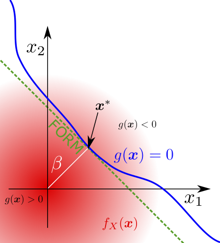
Fig. 5 A diagram of the First Order Reliability Method for two system variables, shown with random variables in the standard normal space.
Second Order Reliability Method
The estimate of the probability of failure obtained from the first order reliability method may be incorrect for nonlinear limit state functions. Therefore, a more accurate quadratic approximation to the limit state surface can be used. This is known as the second order reliability method (SORM).
[113] [114] shows that the probability of failure for quadratic limit state surfaces can be asymptotically approximated by
for large \(\beta\) where \(\kappa_i\) are the principal curvatures of the limit state surface at the design point, which can be obtained either analytically or by using a computational procedure. [115] provides a recent review of the methodology.
The advantage of this method is that it is possible to compute a more accurate estimate of the failure probability than with FORM, and with much lesser computational expense than Monte Carlo sampling. Extraordinarily, the approximation for \(P_f\) becomes more accurate for smaller failure probabilities, i.e. the opposite behaviour of Monte Carlo simulation. The disadvantage of the method is that limit state surfaces which are extremely non-linear will not be approximated well by a quadratic function, and hence the estimated failure probability will be incorrect. This disadvantage can be partially mitigated in some cases by combining multiple SORM estimates at different design points. In addition, in some cases numerically determining the principal curvatures can be problematic due to the additional evaluations of the performance function required relative to FORM.
Line sampling
The fundamental idea behind Line Sampling is to refine estimates obtained from the First-order reliability method (FORM), which may be incorrect due to the non-linearity of the limit state function. Conceptually, this is achieved by averaging the result of different FORM simulations [116]. Firstly, the approximate direction of the failure region from the origin in standard normal space must be determined. This is known as the importance direction. It is usually obtained by finding the design point, by approximate means if necessary. Following this, samples are randomly generated in the standard normal space and lines are drawn parallel to the importance direction in order to compute the distance to the limit state function, which enables the probability of failure to be estimated for each sample.
For each sample of \(\boldsymbol{x}\), the probability of failure in the line parallel to the important direction is defined as: \(P_f(\boldsymbol{x}) = \int^\infty_{-\infty} \mathbb{I}(\boldsymbol{x}+\beta \boldsymbol{\alpha}) d \beta,\) where \(\boldsymbol{\alpha}\) is the importance direction, and \(\phi\) is the probability density function of a Gaussian distribution (and \(\beta\) is a real number). In practice, the roots of a nonlinear function must be found to estimate the partial probabilities of failure along each line. This is either done by interpolation of a few samples along the line, or by using the Newton-Raphson method. The global probability of failure is the mean of the probability of failure on the lines: \(P_f = \frac{1}{N_L} \sum_i^{N_L} P_f^{(i)}\) where \(N_L\) is the total number of lines used in the analysis, and \(P_f^{(i)}\) are the partial probabilities of failure estimated along all the lines.
For problems in which the dependence of the performance function is only moderately non-linear with respect to the parameters modelled as random variables, setting the importance direction as the gradient vector of the performance function in the underlying standard normal space leads to highly efficient Line Sampling. [26] describes enhancements which can be made to Line Sampling to increase the efficiency. For example, the solution of the Newton-Raphson search used on the previous line can be used to inform the search on the next line, if the lines are sorted by proximity. In addition, the importance direction can be updated during simulation based on the completed subset of lines.
The Line Sampling methodology is more expensive than FORM, but far less expensive than Monte Carlo simulation. It is likely to perform poorly for highly non-linear limit state surfaces, but in general offers a good balance between accuracy and computational expense.
Importance sampling
In Importance Sampling, samples are drawn from a distribution with a higher density in the failure region and then re-weighted to obtain a Monte Carlo estimator with reduced variance. The re-weighted estimator is written as
where \(\boldsymbol{x}_i\) are drawn from the proposal density \(h(\boldsymbol{x})\). The optimal proposal density, which results in the greatest reduction of the variance of the estimator is
which is not useful in practice because of the dependence on the quantity to be estimated, \(P_f\). However, the optimal proposal density can be used to motivate the choice of the proposal density in practice. An appropriate \(h(\boldsymbol{x})\) can be chosen by finding the design point with an approximate method and centring the proposal density on the design point, since (29) indicates that the failure region has a higher proposal density. A complete discussion of the technique is given in [117] and [106].
Importance Sampling is useful as it offers an unbiased estimator which can estimate the failure probability with few samples. The main difficultly is determining the proposal distribution \(h(\boldsymbol{x})\). This is usually achieved by engineering judgement and knowledge of the design point.
Subset simulation
Subset simulation aims to calculate \(P_f\) by decomposing the space of the random variables into several intermediate failure events with decreasing failure probability. The conditional probabilities for the intermediate failure regions can then be used to calculate \(P_f\) which is given by \(P_f = P(F_m) = P(F_m) \prod^{m-1}_{i=1} P(F_{i+1}|F_i)\) where \(F_i\) represents intermediate failure event \(i\). By making the conditional probability of samples falling in the intermediate failure regions large, the coefficient of variation of each individual failure event can be minimised, hence minimising the coefficient of variation of \(P_f\). Markov chains are used to generate conditional samples between intermediate failure regions in order to calculate \(P(F_{i+1}|F_i)\). A complete description of the method is given in [118].
The main advantage of Subset Simulation is that it can estimate failure probabilities for non-linear limit state surfaces in a black box manner with relatively low computational expense. However, [119] shows that subset simulation is not accurate for some limit state surfaces, for example limit state surfaces with multiple importance directions.
Metamodels
If inexpensive samples of \(g(\boldsymbol{x})\) or \(\mathbb{I}_f(\boldsymbol{x})\) are available then the estimator \(\hat{P}_f\) can be evaluated trivially. Therefore, the problem of estimating \(P_f\) can be effectively reduced to a machine learning problem. In the case of modelling \(g(\boldsymbol{x})\), the problem is one of regression. In the case of modelling \(\mathbb{I}_f(\boldsymbol{x})\), the problem is classification of the failure region. A machine learning model which fulfils this purpose is known as a metamodel or surrogate model.
In the literature many machine learning techniques have been applied to the reliability analysis problem: linear regression (known as the response surface methodology) [120], support vector machines [121], polynomial chaos expansions [122], neural networks [123] and Gaussian process emulators (sometimes known as Kriging) [124]. Neural networks and Gaussian processes have the advantage of being able to quantify their uncertainty accurately, so the required number of training samples can be assessed. Polynomial chaos expansions allow the sensitivity indices of \(g(\boldsymbol{x})\) to be computed analytically from the trained metamodel [125]. In [126], Interval Predictor Models are used to solve the reliability analysis problem.
In general, the most useful metamodels produce the most accurate estimates of \(P_f\), whilst requiring the smallest number of training samples. An ‘experimental design’ specifies where the samples of \(g(\boldsymbol{x})\) will be made for training. Usually a uniform design is chosen, but other sampling strategies can be used [127]. Active learning can be used to sequentially choose the samples required to train the metamodel. These samples are usually chosen based on where the uncertainty of the metamodel is largest. In adaptive Kriging Monte Carlo simulation (AK-MCS) the samples are chosen at points with large uncertainty, close to the limit state surface. This strategy achieves state of the art efficiency [128]. This strategy is known as active learning, and the function which is used to choose the subsequent sample is known as the probability of misclassification acquisition function.
The main advantage of metamodels is that the estimator for the failure probability based on the metamodel can be made arbitrarily accurate. The main disadvantage is that the metamodel introduces uncertainties, so the problem is effectively shifted to trying to create an accurate metamodel with a small number of samples.
Worked example : First order reliability analysis method (FORM)
For the simple example of a cantilever beam with a point load, \(F\), at any point on the beam, the maximum deflection of the end of the beam is given by \(\delta_{max}=\frac{F a^2}{6 E I} (3l-a)\), where \(I\) is the moment of inertia of the beam, \(a\) is the distance of the point load from the fixed end of the beam, \(l\) is the length of the beam and \(E\) is the modulus of elasticity of the beam [129]. \(E\), \(I\) and \(a\) were fixed, and \(l\) and \(F\) were given by random variables with normal distributions. The chosen values of the parameters are shown below:
Variable |
Distribution |
Mean |
Standard Deviation |
|---|---|---|---|
\(E\) |
Fixed |
200000 N/mm\(^2\) |
N/A |
\(I\) |
Fixed |
78125000 mm\(^4\) |
N/A |
\(l\) |
Normal |
5000 mm |
20 mm |
\(a\) |
Fixed |
3000 mm |
N/A |
\(F\) |
Normal |
30000 N |
20 N |
It is assumed that the beam ‘fails’ when the maximum deflection is greater than 35 mm.
First we need to determine the reliability index (\(\beta\)). This can be achieved by several methods:
# Using optimisation
import scipy.optimize
import numpy as np
from scipy.stats import norm
import matplotlib.pyplot as plt


def deflection(force, distance, elasticity, inertia, length):
    """
    Deflection of a cantilever beam

    Args:
        force: Force
        distance: Distance of the point load from the fixed end of the beam
        elasticity: Modulus of elasticity of the beam
        inertia: Beam moment of inertia
        length: Beam length
    Returns:
        deflection
    """
    return (force * distance ** 2 * (3 * length - distance)
            / (6 * elasticity * inertia))


performance_threshold = 35


def performance(length, force):
    return (performance_threshold
            - deflection(force, 3000, 200000, 78125000, length))


mean_l = 5000
std_l = 20
mean_F = 30000
std_F = 20


def normalise(variable, mean, std):
    """
    Transform variable to standard normal space
    """
    return (variable - mean) / std


def unnormalise(variable, mean, std):
    """
    Transform variable from standard normal space
    """
    return (variable * std + mean)


def transform(length, force):
    return normalise(length, mean_l, std_l), normalise(force, mean_F, std_F)


def inverse_transform(length, force):
    return (unnormalise(length, mean_l, std_l),
            unnormalise(force, mean_F, std_F))


results = scipy.optimize.minimize(
    lambda x: np.linalg.norm(x),
    x0=[0, 0],
    constraints=scipy.optimize.NonlinearConstraint(
        lambda x: performance(*inverse_transform(*x)), lb=0, ub=0),
)
beta = results.fun
design_point = results.x
P_f = norm.cdf(-beta)
print(P_f)
0.0058112134307528535
# Using gradient of performance function

def gradient_performance_function_lf(force, distance, elasticity, inertia,
                                     length):
    """
    Gradient of performance function with respect to l and F

        Args:
        force: Force
        distance: Distance of the point load from the fixed end of the beam
        elasticity: Modulus of elasticity of the beam
        inertia: Beam moment of inertia
        length: Beam length
    """
    dg_dl = -3 * force * distance ** 2 / (6 * elasticity * inertia)
    dg_dF = -distance ** 2 * (3*length - distance) / (6 * elasticity * inertia)
    return np.array([dg_dl, dg_dF])


def unnormalised_gradient_at_mean(length, force):
    return gradient_performance_function_lf(force, 3000, 200000, 78125000,
                                            length)


gradient_at_mean = unnormalised_gradient_at_mean(
    *inverse_transform(mean_l, mean_F))
importance_direction = - gradient_at_mean / np.linalg.norm(gradient_at_mean)
beta = performance(mean_l, mean_F) / np.linalg.norm(gradient_at_mean)
design_point = importance_direction * beta
P_f = norm.cdf(-beta)
print(P_f)
0.008363326195416835
# Check result using Monte Carlo
n_samples = 1000000
samples_standardised = np.random.randn(n_samples, 2)
samples_l, samples_F = inverse_transform(
    samples_standardised[:, 0], samples_standardised[:, 1])
P_f = np.mean(performance(samples_l, samples_F) < 0)
print(P_f)
0.005767
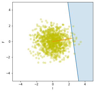
Below, a plot is shown of the model:
def limit_state_F(length, distance, elasticity, inertia):
    """
    Parametric equation for limit state surface for F as a function of l
    """
    return 35 / (distance ** 2 * (3 * length - distance)
                 / (6 * elasticity * inertia))


# Plot the limit state surface - where performance function is zero
x_plot = np.arange(-10, 10)
unnormalised_x = unnormalise(x_plot, mean_l, std_l)
limit_state = limit_state_F(unnormalised_x, 3000, 200000, 78125000)
normalised_limit_state = normalise(limit_state, mean_F, std_F)
plt.plot(x_plot, normalised_limit_state)
# Shade failure region - to the right of limit state surface
# (performance function < 0)
plt.fill_between(x_plot, normalised_limit_state, 5, alpha=0.2)

# Plot some samples from the Monte Carlo simulation
n_samples_to_plot = 1000
plt.scatter(
    samples_standardised[:n_samples_to_plot, 0],
    samples_standardised[:n_samples_to_plot, 1],
    alpha=0.3, color="y"
)

# Plot beta - the line linking design point with the origin
plt.plot([0, design_point[0]], [0, design_point[1]])

# Set plot properties
fig = plt.gcf()
fig.set_size_inches(5, 5)
plt.xlim(-5, 5)
plt.ylim(-5, 5)
plt.xlabel("l")
plt.ylabel("F")
plt.show()