Set-based models of uncertainty
The two most common set-based models of uncertainty are convex sets and interval models. The popularity of these models can be attributed to the computational simplifications they enable, relative to non-convex set models of uncertainty. Set-based models are a method of characterising uncertainty, without describing the level of belief for each distinct value, as in probabilistic models. Alternatively, they can be seen as an initial way of prescribing the support for an as-yet undetermined probabilistic model.2
Interval models of uncertainty
An interval model of uncertainty is a set of numbers where any number falling between the upper and lower bounds of the interval is included in the set. In the interval notation, an interval uncertainty model is given by \(X = [\underline{x}, \overline{x}] = \{x \in \mathbb{R} \mid \underline{x} \le x \le \overline{x} \}\) [39]. Note that interval models can also be defined for the case where the endpoints are excluded from the intervals, and in this case regular brackets are used instead of square brackets. Interval models can be re-parameterised in terms of their centre and interval radius, \(c = \frac{\overline{x} + \underline{x}}{2}\) and \(r = \frac{\overline{x} - \underline{x}}{2}\). Interval models usually don’t express dependency between multiple variables.
Note that when using an interval model of uncertainty, the relative likelihoods of different values of the variable are unknown and therefore it is impossible to draw precise samples from the model in the same sense that one draws samples from a probability distribution. Put simply, an interval model represents complete lack of knowledge, apart from the bounds. For this reason, they are often preferred for modelling severe epistemic uncertainty, sometimes known as incertitude, rather than aleatory uncertainty, where the ability to model the variability of a quantity is the main focus [40].
Basic computation with interval models is typically computationally inexpensive since one can rely upon interval arithmetic for elementary operations. Complex functions and computer codes can be ‘converted’ to accept interval inputs by applying the so-called natural extension, where arithmetic operations are converted to interval arithmetic and real valued inputs are replaced with interval values [39]. However, applying the natural interval extension can result in gradual widening of the prediction interval during propagation through the code, due to repeated appearance of the same variables [39].
In many cases, one can create a Taylor expansion for \(g(x)\) up to terms of a specific order in \(x\), and then use an interval bound for the rounding error to rigorously and accurately bound \(g(x)\) [41] [42] [43]. Intermediate linear Taylor models may be combined together to yield relatively tight bounds on the output with reduced computational expense, since computing the maximum of a multivariate linear function over a set of intervals is trivial. Engineers could choose to neglect the modelling of the remainder in cases where a rigorous bounding of the range of \(g(x)\) over \(X\) is not required, or the Taylor model is sufficiently accurate. Alternatively, if \(g(x)\) is represented a Bernstein polynomial, bounds on the range of \(g(x)\) over \(X\) can be obtained analytically [44].
For complex functions or computer codes it may not be possible to rewrite the code in terms of interval arithmetic, as the code may be ‘black-box’ and therefore inaccessible. In these cases it may be necessary to rely upon numerical optimisation to compute approximate bounds on the range of \(g(x)\). For example, if one wishes to make predictions about the output of a model \(g(x)\) for \(x \in [\underline{x}, \overline{x}]\) then one must evaluate
For general \(g(x)\), a non-linear optimiser with the ability to respect bounds must be used to solve (3), for example Bayesian optimisation or a genetic algorithm. A brute force search could also be used to solve (3). If \(g(x)\) is convex, then one may apply convex optimisation routines [45]. Due to the curse of dimensionality this optimisation becomes more difficult when there are many interval variables to be propagated, since the complexity for many convex optimisation algorithms increases with the dimensionality of the problem [46].
The method of Cauchy deviates offers an efficient alternative to computing finite difference gradients of \(g(x)\) in order to apply a Taylor expansion for black-box functions [47]. The Cauchy deviates method evaluates \(g(x)\) for a set of transformed samples drawn from Cauchy distributions and then uses the property that the linear combination of Cauchy distributed random variables is also Cauchy distributed with a known distribution parameter to bound \(g(x)\).
Worked example : Interval Models
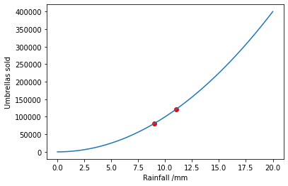
This time, the model of rainfall will be given by an interval. Imagine the rainfall in London on a particular day is known to be bounded in the interval \(x \in [9, 11]\).
Again the number of umbrellas sold is given by \(1000 x^2\).
To bound the number of umbrellas sold we must evaluate \([\min_{x \in [9, 11]} 1000 x^2, \max_{x \in [9, 11]} 1000 x^2]\)
This can be evaluated analytically since \(x^2\) is monotonic in \(x\) for positive \(x\):
import numpy as np
import matplotlib.pyplot as plt
import scipy.optimize


def g(x): return 1000 * x ** 2


min_x = 9
max_x = 11

umbrellas_sold = [g(min_x), g(max_x)]
print("The number of umbrellas sold falls in the interval: {}".format(
    umbrellas_sold))

x_grid = np.linspace(0, 20, num=200)
plt.plot(x_grid, g(x_grid))
plt.scatter([min_x, max_x], g(np.array([min_x, max_x])), color="red")
plt.xlabel("Rainfall /mm")
plt.ylabel("Umbrellas sold")
plt.show()
The number of umbrellas sold falls in the interval: [81000, 121000]
This can also be evaluated approximately using a taylor series (shown in green):
def g_dash(x): return 1000 * 2 * x


x_mid = (max_x + min_x) / 2


def taylor_expansion(x): return g(x_mid) + (x - x_mid) * g_dash(x_mid)


x_grid = np.linspace(0, 20, num=200)
plt.plot(x_grid, g(x_grid))
plt.plot(x_grid, taylor_expansion(x_grid), color="green")
plt.scatter([min_x, max_x], g(np.array([min_x, max_x])), color="red")
plt.xlabel("Rainfall /mm")
plt.ylabel("Umbrellas sold")
plt.show()

umbrellas_sold = [taylor_expansion(min_x), taylor_expansion(max_x)]
print("The number of umbrellas sold falls in the interval: {}".format(
    umbrellas_sold))
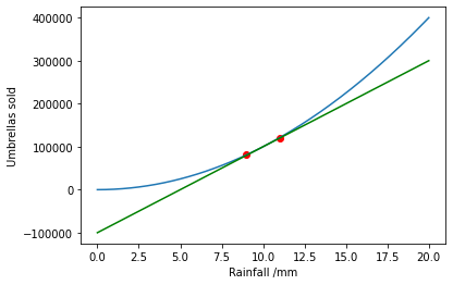
The number of umbrellas sold falls in the interval: [80000.0, 120000.0]
Finally we use black box optimisation in scipy.optimize to evaluate the interval model:
min_umbrellas = scipy.optimize.minimize(g, x0=x_mid, bounds=[(min_x, max_x)])
neg_max_umbrellas = scipy.optimize.minimize(lambda x: -g(x),
                                            x0=x_mid,
                                            bounds=[(min_x, max_x)])
print("The number of umbrellas sold falls in the interval: {}".format(
    [min_umbrellas.fun[0], -neg_max_umbrellas.fun[0]]))
The number of umbrellas sold falls in the interval: [81000.0, 121000.0]
Convex set models of uncertainty
A convex set is defined as a set where, for any two points in the set, all points along the connecting line between the two points are also included in the set. Convex sets are useful as they are in many ways similar to interval models, but allow dependencies to be modelled between variables. [48] provide examples of how convex set models may be used in engineering practice. There is a deep connection between interval models and convex set models. An interval model with multiple variables would be represented as the specific case of a hyper-rectangular convex set. In addition, affine transformations of hyper-rectangular convex sets result in a class of models known as zonotopes [49].
The smallest convex set containing a particular set of data points is termed the convex hull of the dataset. Computing the convex hull of a dataset has complexity \(\mathcal{O}(n\log{n} + n^{\lfloor \frac{d}{2} \rfloor})\) [50], where \(\lfloor \cdot \rfloor\) is the floor operator which rounds a real number down to the nearest integer, and therefore in practice one often learns a simplified representation of the convex set with desirable computational properties.
\(\ell_p\) ellipsoids (for \(p>1\)) are a particularly useful case of a convex set, because they can be easily manipulated in calculations [51]. An \(\ell_p\) ellipsoid is given by the set \(X = \{ x \mid \left\| x - c\right\| _{p, w} \le r \}\), where the weighted \(\ell_p\) norm is \(\left\| x \right\| _{p, w} = (\sum^{N}_{i=1} |w_i x_i|^p)^{\frac{1}{p}}\), \(x_i\) are variables in a set of dimensionality \(N\), \(c\in\mathbb{R}^N\) represents the centre point of the set, and \(w_i\) are weights controlling the relative uncertainty in each variable [52]. \(p\) can be adjusted to control the correlation between the variables. The case \(\ell_\infty\) corresponds to the hyper-rectangle (interval) model, where there is no correlation between variables. When \(p\) is decreased the variables become more correlated.
Computation with convex set models is performed in the same way as with interval models, except the bounds on \(x\) are replaced with convex constraints:
where \(X\) is a convex set. If \(g(x)\) is linear with known gradient, and \(X\) is a hyper-sphere or hyper-rectangle, then this optimisation program in (4) admits an analytic solution [53]. If the convex set is small then the analytic solution may be a reasonable solution when used with a Taylor expansion for \(g(x)\), as with interval uncertainty models.
- 2
The support of a distribution is the set of values for which the probability measure is non-zero.